
Vignette#
This vignette derives BCMP domains from an unintegrated single-cell dataset, then uses these domains to rank candidate integration methods.
# If needed: python -m pip install matplotlib
import matplotlib.pyplot as plt


from bcmp import bcmp
from bcmp.datasets import diabetic_kidney_lite
1. Load the AnnData input#
The bundled example contains raw counts and batch labels in obs["batch"].
adata = diabetic_kidney_lite()
print(adata)
AnnData object with n_obs × n_vars = 1500 × 27980
    obs: 'batch'
    uns: 'integration_benchmark'
    obsm: 'X_CSS', 'X_ComBat', 'X_Harmony', 'X_LIGER', 'X_Scanorama', 'X_Seurat_cca', 'X_Seurat_rpca', 'X_Uncorrected', 'X_demo_umap', 'X_fastMNN', 'X_scANVI', 'X_scVI'
2. Run BCMP#
Simply run BCMP with the AnnData object and its batch key:
result = bcmp(
    adata,
    batch_key="batch",
    verbose=False,
)
adata_bcmp = result.adata
print(adata_bcmp)
AnnData object with n_obs × n_vars = 1500 × 27980
    obs: 'batch', 'bcmp_domain'
    uns: 'integration_benchmark'
    obsm: 'X_CSS', 'X_ComBat', 'X_Harmony', 'X_LIGER', 'X_Scanorama', 'X_Seurat_cca', 'X_Seurat_rpca', 'X_Uncorrected', 'X_demo_umap', 'X_fastMNN', 'X_scANVI', 'X_scVI'
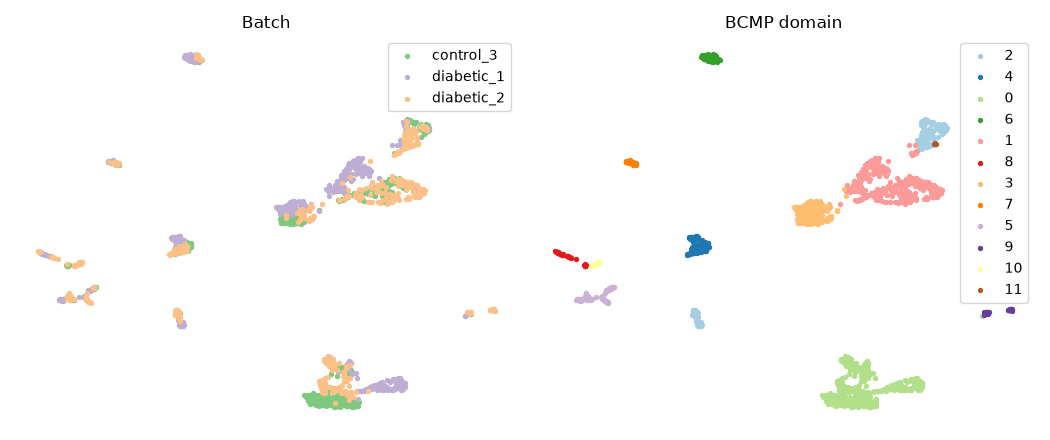
The resulting domains can be visualized as follows:
coordinates = adata_bcmp.obsm["X_demo_umap"]

_, axes = plt.subplots(1, 2, figsize=(10.5, 4.4))
for axis, key, title, palette in zip(
    axes,
    ["batch", "bcmp_domain"],
    ["Batch", "BCMP domain"],
    [plt.get_cmap("Accent"), plt.get_cmap("Paired")],
):
    labels = adata_bcmp.obs[key].astype(str)
    for index, label in enumerate(labels.unique()):
        axis.scatter(
            *coordinates[labels.eq(label).to_numpy()].T,
            s=8,
            color=palette(index),
            label=label,
        )
    axis.set_title(title)
    axis.set_axis_off()
    axis.legend()

plt.tight_layout()
plt.show()
3. Rank candidate integration methods#
The bundled candidate embeddings are stored in obsm. Their keys and
display names are recorded in uns["integration_benchmark"].
benchmark = adata_bcmp.uns["integration_benchmark"]
embedding_keys = benchmark["embedding_keys"].tolist()
method_names = benchmark["method_names"]
BCMP domains are supplied as the population labels for every candidate embedding.
from scib_metrics.benchmark import BatchCorrection, Benchmarker

benchmarker = Benchmarker(
    adata_bcmp,
    batch_key="batch",
    label_key="bcmp_domain",
    embedding_obsm_keys=embedding_keys,
    bio_conservation_metrics=None,
    batch_correction_metrics=BatchCorrection(),
    n_jobs=1,
    progress_bar=False,
)
benchmarker.benchmark()
ranking = (
    benchmarker.get_results(min_max_scale=True)
    .drop(index="Metric Type")["Batch correction"]
    .astype(float)
    .sort_values(ascending=False)
)
ranking.index = [method_names[key] for key in ranking.index]
ranking.index.name = "Method"
print(ranking.round(2).to_string())
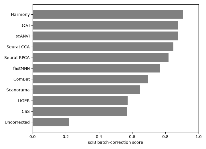
Method
Harmony        0.91
scVI           0.88
scANVI         0.87
Seurat CCA     0.85
Seurat RPCA    0.82
fastMNN        0.77
ComBat         0.69
Scanorama      0.65
LIGER          0.57
CSS            0.57
Uncorrected    0.22
A bar plot provides another view of the ranking:
_, score_ax = plt.subplots(figsize=(7.2, 5.2))
score_ax.barh(ranking.index, ranking, color="0.5")
score_ax.set(xlabel="scIB batch-correction score", xlim=(0, 1), ylabel="")
score_ax.invert_yaxis()
plt.tight_layout()
plt.show()